Background information module celestial
Rotation matrices
Spherical astronomy sections in older textbooks rely heavily on the reader’s knowledge of spherical trigonometry (e.g. Smart 1977). For more complicated problems than a simple rotation, this technique becomes laborious. Matrix and vector techniques come to rescue. Many of the transformations are defined in terms of rotation matrices. A rotation matrix is a matrix whose multiplication with a vector rotates the vector while preserving its length. There is a special group 3 x 3 rotation matrices R where
For transformations between sky systems we only use matrices with \(|R|=+1\).
A coordinate rotation is a rotation about a single coordinate axis. The three coordinate rotation matrices are:
Three coordinate rotations in sequence can describe any rotation. The result matrix is:
The angles are called Euler angles. There are 27 possible sequences of the three indices i,j,k. Not all sequences are valid rotations. The most common choices of valid combinations are (1,2,3), (3,1,3) and (3,2,3) ( [Diebel], 2006)
If \(\vec r_0\) is a position vector in system 0 and \(\vec r_1\) is the same position in the sky but in another sky system then, with the appropriate rotation matrix R, we calculate \(\vec r_1\) in the coordinates belonging to the rotated system with:
Note that the listed rotations represent the same position in different coordinate systems. The indices 1,2,3 correspond to the rotation axes x, y, z. In this documentation we will write \(R_x\) for \(R_1\), \(R_y\) for \(R_2\) and \(R_z\) for \(R_3\):
If (\(\alpha,\delta\)) is the longitude and latitude of a position in system 0, then the corresponding position vector can be written as:
Note that the longitude and latitude applies to the other sky systems too, but then we use other symbols, like (\(\lambda, \beta\)), (l,b) or (sgl, sgb). From any position (x,y,z) we calculate the longitude and latitude with the expressions:
and
where we used the arctan2 function to solve for (lon,lat) to keep the right quadrant. Longitudes range from \(0^\circ\) to \(360^\circ\) and latitudes from \(-90^\circ\) to \(90^\circ\).
FK4
The impression one could get from the literature is that FK4 and FK4-NO-E are different sky systems and that there exists a matrix to rotate a position from one system to the other. But this is not true. The systems differ because positions in FK4 catalogs usually contain the elliptic terms of aberration (so they are almost mean places). Others list positions that are corrected for these E-terms (like catalogs with radio sources). Also B1950 radio interferometer data (e.g. maps from the W.S.R.T.) could be processed in a way that positions are corrected for E-terms. It is convenient to define a system that is FK4 but without the E-terms. FITS uses the name FK4-NO-E for this system. Catalog positions corrected for the E-terms are (real) mean places and are used for precession and transformations from FK4 B1950 positions to FK5 J2000 positions and galactic coordinates.
In a later section we give the original definition of galactic coordinates.
FK4 and the elliptic terms of aberration
Stellar aberration is caused by the motion of the earth in its orbit. This motion is represented by a circular velocity component and a component perpendicular to the major axis caused by the fact that the orbit is elliptical. This velocity component is responsible for elliptical terms of aberration (E-terms) which are less than 0.35 arcseconds (maximum is equal to the constant of aberration times the eccentricity of the earths orbit = 20”.496 x 0.01673 ~= 343 mas). The terms are independent of the position of the earth and depend only on the position of the object in the sky.
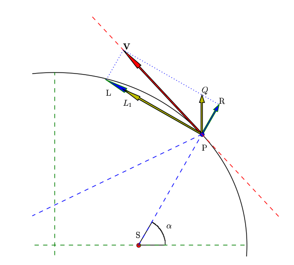
Fig.1 – Ecliptic from above showing e-terms.
Fig.1 shows the ecliptic from above.
S is the Sun, in one of the focal points of the ellipse and P the position
of the Earth. The plot was made with Python script etermfig.py.
Smart (1977) gives an excellent description of aberration and its elliptical terms. We reproduced one of his figures with a small program. Here are the steps.
Given an elliptical orbit with semi major axis a and semi minor axis b, and center at (0,0), the positions of the focal points are (-c,0) and (c,0) with \(c^2 = a^2 - b^2\)
Suppose the Sun is in focal point S and the Earth is on the ellipse in P
The tangent in P is the normal of the bisector of the two lines from focal point to P
r is the radius vector SP
Earth has a velocity V along the tangent at P and:
(11)\[ V^2 = {PL}^2 + {PR}^2 = ({\frac{dr}{dt}})^2 + ({r\frac{d\alpha}{dt}})^2\]So for given P and a velocity V, we can calculate the angle between the normal of SP (i.e. in the direction PL) and decompose V into a linear velocity perpendicular to the radius vector and a component in the direction of the radius vector
Now we want to decompose V into a circular velocity component \(PL_1\) and a velocity perpendicular to the major axis (PQ)
\(PQ = PR / \sin(\alpha)\) and \(PL_1 = PL - PR / \tan(\alpha)\)
Smart derives two epressions:
with:
With M is mass of the Sun, m is mass of the Earth, G is the gravitational constant and e is the eccentricity of the ellipse:
The most important observation now is that these velocities are constant! Therefore the total displacement of the position of a star due to aberration can be decomposed into a displacement due to a constant velocity at right angle to the radius vector and one due to a constant velocity perpendicular to the major axis.
If the position of a star is given by longitude \(\lambda\) and latitude \(\beta\) and the longitude (measured from the vernal equinox) is \(\omega\) then the displacements due to the velocity perpendicular to the major axis are:
and \(\kappa\) is the constant of aberration (Smart section 108).
The constant of aberration is defined as:
and c is the speed of light.
The value of \(\kappa\) is 20”.496. Therefore, given the eccentricity of the Earth’s orbit (0.01673), the maximum displacement in \(\lambda\) or \(\beta\) is 20”.496 * 0.01673 ~= 343 mas.
Data in FK4 catalogs are ‘almost’ mean places because the conventional correction for annual aberration in FK4 includes only terms for circular motion and not the small E-terms. Therefore all published FK4 catalog positions are affected by elliptic aberration.
Mean places should be unaffected by aberration of any kind. Thus, for precession or transformation of FK4 positions, one should remove the E-terms first.
With a standard transformation from ecliptic coordinates to equatorial coordinates one can find expressions for the displacements in \(\alpha\) and \(\delta\). (e.g. see ES, section 3.531, p 170):
where \(\epsilon\) is the obliquity of the ecliptic.
Also one could write a position vector in an equatorial system:
and a second vector:
then one can define the E-term vector as:
If one works out this difference between two vectors, neglect terms that are very small and rearrange the equations so that we can compare them to the expressions for the displacements in \(\alpha\) and \(\delta\), then the E-term vector is equal to:
This E-term vector can then be used to transform FK4 positions to real mean places (i.e. remove E-terms) or to convert mean places to FK4 catalog positions (i.e. add E-terms).
Module celestial calculates the E-term vector in the equatorial system as function of
epoch.
Removing and adding E-term vectors are best illustrated in a figure.
In the next plot, the red circle represents the FK4 catalog system.
For each unit vector in this circle one can transform a position in RA, Dec to
a new position where the E-terms are removed. The new vector has its end point on the
blue circle. So adding E-terms would be as simple as adding the E-term vector to
the new vector. However, if one converts the new position to RA and Dec, the information
about the length of the new vector will be lost. If one converts these RA and Dec
back to Cartesian coordinates, and add the E-term vector, then we would not obtain the
original vector that we started with. Plot and explanation demonstrate how we
should deal with removing and adding E-terms:
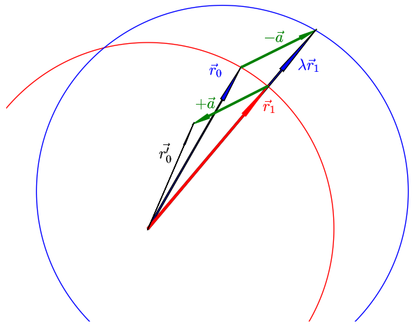
Fig.2 – E-term vectors.
In the figure one starts with a FK4 catalog position represented by vector \(\vec r_0\). Removing the E-terms (represented by vector \(\vec a\)) results in vector \(\lambda \vec r_1\). If vectors kept their length after converting them back to longitude and latitude then the inverse procedure would be as easy to add vector \(\vec a\) to \(\lambda \vec r_1\). Usually this is not the case, so for convenience we normalize \(\lambda \vec r_1\) to get unit vector \(\vec r_1\).
However, if we add vector \(\vec a\) to \(\vec r_1\) we end up with a vector \(\vec {r'}_0\) which is not aligned with the original vector. To get it aligned, we have to stretch \(\vec r_1\) again with some factor \(\lambda\). We need an E-term adding procedure that applies to all unit vectors. It is straightforward to derive an expression for the wanted scaling factor \(\lambda\):
Adding the E-term vector applying the conditions described above we write:
And the conditions are:
If we write this out in terms of the Cartesian coordinates x, y, z then with \(\vec r_1 = (x_1,y_1,z_1)\), \(\vec r_0 = (x_0,y_0,z_0)\), and \(\vec a = a_x,a_y,a_z)\):
And:
If we substitute the expressions for \(\vec r_0\) (25) in this last equation (eq.27) then we obtain the simplified expression for \(\lambda\):
with:
We know that the length of the E-term vector a is much smaller than 1 so p is always less than 0. We also observe that only the positive solution for \(\lambda\) is the one we are searching for because a negative value represents a vector in opposite direction. Then we are left with an expression for the wanted \(\lambda\):
We started with known \(\vec r_1\) and \(\vec a\). With those we can calculate the wanted vector \(\vec r_0\), which represents the catalog position.
Transformations between the reference systems FK4 and FK5
For conversions between FK4 and FK5 we follow the procedure of Murray [Murray]. Murray precesses from B1950 to J2000 using a precession matrix by Lieske (1979) and then applies the equinox correction and ends up with a transformation matrix X(0) and its rate of change per Julian century X’(0).
If F is the ratio of Julian century to tropical century (1.000021359027778) and T is the time in Julian centuries from the epoch B1950, then Murray derives a transformation equation for a position and velocity in FK4:
Positions:
If the epoch of observation is T in Julian centuries counted from B1950 then from the previous equation we derive:
Module celestial assumes that we have unknown or zero proper motions. We allow for
fictitious proper motion in FK5, then we get the equation:
where v is the (fictitious) proper motion in FK5 and t is the time in Julian
centuries form J2000.
This is how the function celestial.FK42FK5Matrix() works for a given epoch of
observation. In the output of the next interactive session, we show the results
of varying the epoch of observation for a position R.A., Dec = (0,0):
>>> from kapteyn.celestial import *
>>> print sky2sky( (eq,'b1950',fk4), (eq,'j2000',fk5), 0,0)
[[ 0.640691    0.27840944]]
>>> print sky2sky( (eq,'b1950',fk4, 'J1970'), (eq,'j2000',fk5), 0,0)
[[ 0.64070422  0.27838524]]
>>> print sky2sky( (eq,'b1950',fk4, 'J1980'), (eq,'j2000',fk5), 0,0)
[[ 0.64071084  0.27837314]]
>>> print sky2sky( (eq,'b1950',fk4, 'J1990'), (eq,'j2000',fk5), 0,0)
[[ 0.64071745  0.27836105]]
The differences are a result of the fact that FK4 is slowly rotating with respect to the inertial FK5 system.
Velocities
The relation between velocities in the two systems is given also by the transformation equations:
Then:
Module celestial deals with positions from maps with objects for which we expect that
the proper motion in FK5 is zero (e.g. extra-galactic sources). Then the expression for
the fictitious proper motion in FK4 is:
If we substitute this in equation (33) then we have the simple relation:
To summarize the possible transformations between FK4 and FK5:
Note
If you allow non zero proper motion in FK5 you should specify an epoch for the date that the mean place was correct and apply the formula:
If you are sure that the your position corresponds to an object with zero proper motion in FK5 then the epoch of observation is not necessary and one applies the formula:
Note that the matrix X(0) is not a rotation matrix because the inverse matrix is not equal to the transpose. Therefore the transformation matrix for conversion of FK5 to FK4 is the inverse of X(0).
Murray’s method has been described as controversial (e.g. see Soma (1990), [Soma]), but Poppe (2005) [Poppe] shows that the differences in results between the methods of Standish, Aoki and Murray are less than 5 mas.
Radio maps
Much of the B1950 data that users at the Kapteyn Astronomical Institute transform to FK5 J2000, is data from the Westerbork Synthesis Radio Telescope (WSRT). For this telesope we retrieved some information about the correction program that was used to transform apparent places to mean places. Apparent coordinates change during an observing run, due to:
Refraction
Precession
Nutation
- Aberration
- Annual aberration
- Diurnal aberration
- Secular aberration (unknown and not significant)
- Planetary aberration (unknown and not significant)
Proper motion (not significant)
Parallax (not significant)
If \(X_t\) are the coordinates of a source at a time t, \(X_e\) are the coordinates at epoch e and:
- N is the rotation matrix describing the nutation
- P is the rotation matrix describing the precession
- A is the vector describing the annual aberration
- D is the vector describing the diurnal aberration
then the following relations apply:
The vector describing the correction for annual aberration is the vector
C and D are the so called Besselian Day Numbers (tabulated in the Astronomical Almanac) that correct for annual aberration. Early interferometers like the WSRT produced images with greater resolution than obtainable in the optical at that time and in the construction of the radio maps a correction for the elliptical terms was included. So these maps are in fact FK4-NO-E (which is FITS terminology for a FK4 map where the E-terms are removed). For precession and transformations for these maps, no E-terms need to be removed.
Regretably many of FITS files with B1950 data do not include a value for the RADESYS keyword
and one should try to find out how the coordinate system of these radio maps were
constructed to be sure whether E-terms are included or not.
Calabretta (2002) writes:
FK4 coordinates are not strictly spherical since they include a contribution from the elliptic terms of aberration, the so-called E-terms which amount to a maximum of 343 milliarcsec. Strictly speaking, therefore, a map obtained from, say, a radio synthesis telescope, should be regarded as FK4-NO-E unless it has been appropriately resampled or a distortion correction provided. In common usage, however, `CRVAL` for such maps is usually given in FK4 coordinates. In doing so, the E-terms are effectively corrected to first order only.
Contradictory to this, we understand that it depends on how a radio map is sampled whether E-terms are included or not. Also not clear is the reason why one would resample a map in FK4-NO-E. Finally, assuming that usually CRVAL is given in FK4 coordinates seems a bit dangerous. For example for a transformation to Galactic coordinates the E-terms in the FK4 map are removed while it possibly didn’t contain E-terms at all.
With a primary focus on maps with extragalactic objects we have to be sure that galaxy positions given in FK4 coordinates can reliably be converted to FK5 positions. Cotton (1999) [Cotton] presents a list with galaxy positions in B1950 and J2000 coordinates from the Uppsala General catalog (UGC). For the J2000 positions they used Digitized Sky Survey (DSS) images to measure accurate positions of all included UGC galaxies. The positions are accurate to the arcsecond level. For a sample of these galaxies we converted the B1950 positions and compared these to the listed J2000 positions in the article. The numbers were accurate to 10 mas, well within the positional errors given in the listing (which are > 1 arcsecond).
For VLBI data we need another kind of test for accuracy. Aoki (1986) [Aoki2] compares the transformation results of the B1950 position of 3C273B
\(\alpha=12^h26^m33.246^s\), \(\delta=2^\circ 19^\prime 42^{\prime \prime}.4238\), epoch of observation: 1978.62) to J2000 of several authors. He concludes that different authors use different methods and get different results. Aoki’s method differs a few tens mas from the J2000 (VLBI radio sources based) catalog position where RA=12h29m6.6997 (no value for Dec was given). We also noticed that the highest accuracy is obtained if one uses the epoch of observation. Aoki’s result differs 1.6 mas from the catalog value. The results of celestial.py differ only 0.01 mas in RA compared to Aoki’s results.
Hering (1998) [Hering] gives a short description of a procedure in which a B1950 position of a radio source is converted to a J2000 position using the position in B1950 and J2000 of a calibrator source assuming that the angular distance between these sources is the same in both reference systems. An example of Radio star HIP 66257 was added:
1 2 3 4 5 6 7 8 9 10 11 12 13 14 | Calibrator: 1404+286 (FK4)
alpha(B1950) = 14h 04m 45.613s delta(B1950) = 28d 41' 29.22''
1404+286 (ICRF)
alpha(J2000) = 14h 07m 00.3944s delta(J2000) = 28d 27' 14.690''
Radio star: HIP 66257 = HR 5110, Julian epoch of observation: t0 = 1982.3619
alpha(B1950) = 13h 32m 32.145s delta(B1950) = 37d 26' 16.18''
Updated radio star position with respect to the calibrator given
in the ICRF:
alpha(J2000) = 13h 34m 45.6817s delta(J2000) = 37d 10' 56.854''
Celestial: FK4 to ICRS
alpha(J2000) = 13h 34m 45.6862s delta(J2000) = 37d 10' 56.790''
|
We assumed that the original article has an error in the value of alpha(J2000)
of 2 seconds. This must be a typing mistake because the procedure described in that article
is based on Aoki (1986) and when we apply this method to the data we are close to
the corrected position. A difference of 2000 mas cannot be explained otherwise.
The difference between celestial and the updated radio star position
using the method of constant angular distances, is:
\((\Delta \alpha, \Delta \delta) = (68\ mas, 64\ mas)\)
Hering claims a difference between the updated radio star position and that obtained by (his) formal transformation from B1950 to J2000 of:
\((\Delta \alpha \cos(\delta), \Delta \delta) = (20\ mas, 7\ mas)\)
It is not straightforward to draw conclusions from these comparisons because the
formal transformation is not described in detail. The results of celestial
are close to Aoki’s so if Hering’s method is based on Aoki’s, we expect
comparable differences, which is, for unknown reasons, not the case.
Galactic Coordinates
According to Blaauw et al. (1959), the original definitions for the Galactic sky systems are:
The new north galactic pole lies in the direction:
(44)\[(\alpha,\ \delta) = (12h49m\ ,\ 27^\circ .4) = (192^\circ .25,\ 27^\circ .4)\](equinox 1950.0)
The new zero of longitude is the great semicircle originating at the new north galactic pole at the position angle theta = 123 degrees with respect to the equatorial pole for 1950.0.
Longitude increases from 0 degrees to 360 degrees. The sense is such that, on the galactic equator increasing galactic longitude corresponds to increasing Right Ascension. Latitude increases from -90 degrees through 0 degrees to +90 degrees at the new galactic pole.
Given the RA and Dec of the galactic pole, and using the Euler angles scheme Rz(a3).Ry(a2).Rz(a1), we first rotate the spin vector of the XY plane about an angle a1 = 192.25 degrees and then rotate the spin vector in the XZ plane (i.e. around the Y axis) with an angle a2 = 90-27.4 degrees to point it in the right declination.
Now think of a circle with the galactic pole as its center. The radius is equal to the distance between this center and the equatorial pole. The zero point in longitude now is opposite to this pole We need to rotate along this circle (i.e. a rotation around the new Z-axis) in a way that the angle between the zero point and the equatorial pole is equal to 123 degrees. So first we need to compensate for the 180 degrees of the current zero longitude, opposite to the pole. Then we need to rotate about an angle 123 degrees but in a way that increasing galactic longitude corresponds to increasing Right Ascension which is opposite to the standard rotation of this circle (note that we rotated the original X axis about 192.25 degrees which flips the direction of rotation when viewed from (0,0,0). The last rotation angle therefore is a3 = 180-123 degrees. The composed rotation matrix is calculated with:
The numbers are the same as in Slalib’s ‘ge50.f’
and in the matrix of eq. (32) of Murray (1989) [Murray].
The numbers in the composed rotation matrix to convert equatorial FK4 mean places to IAU1958
galactic coordinates, calculated with celestial are:
>>> from kapteyn.celestial import *
>>> import numpy
>>> m = skymatrix((eq,'b1950',fk4), gal)[0]
>>> print numpy.array2string(numpy.array(m), precision=12)
[-0.066988739415 -0.872755765852 -0.483538914632]
[ 0.492728466075 -0.45034695802   0.744584633283]
[-0.867600811151 -0.188374601723  0.460199784784]
Compare this to the numbers in SLALIB’s ge50.f:
[-0.066988739415D0,-0.872755765852D0,-0.483538914632D0]
[+0.492728466075D0,-0.450346958020D0,+0.744584633283D0]
[-0.867600811151D0,-0.188374601723D0,+0.460199784784D0]
And to Murray’s matrix:
[-0.066988739 -0.872755766 -0.483538915]
[ 0.492728466 -0.450346958  0.744584633]
[-0.867600811 -0.188374602  0.460199785]
FK4 catalog positions are not corrected for the elliptic terms of aberration. One should remove these terms first before transforming to galactic coordinates.
Transformations from FK5 J2000 to Galactic coordinates
Galactic coordinates are defined using features in the FK4 system. If these axes could be identified with catalog objects one should first remove the E-terms. Then the rotation to FK5 results in a new system of axes that are non-orthogonal because the E-term correction depends on the position in the sky. Therefore we consider the position of the galactic pole as a FK4 position corrected for E-terms (i.e. FK4-NO-E) and apply transformations only to FK4 positions corrected for E-terms (i.e. we transform from and to the FK4-NO-E system). According to Blaauw (private communication 2008) the precision in the determination of the position of the galactic pole did not justify the effort to bother about E-terms. So if we define the position of the Galactic pole to be in FK4-NO-E coordinates, we don’t change the original definition.
Using this definition of the galactic pole one can find the position of this pole in J2000 coordinates by direct transformations from FK4-NO-E to FK5 and define a rotation matrix for a transformation from FK5 to Galactic coordinates. But to preserve as accurate as possible the galactic coordinates of objects observed in the FK4 system one should first apply the transformation from FK5 to FK4-NO-E and then apply the transformation from FK4-NO-E to Galactic coordinates.
We identify the same problem with the conversion from FK4 to Ecliptic coordinates and using the same logic, we only define transformation between FK4-NO-E and the Ecliptic system.
Note
Transformations involving FK4 coordinates are defined in the FK4-NO-E system. For FK4 catalog positions, this means that one needs to remove the E-terms first before any transformation is applied.
The composed rotation matrix for FK5 to Galactic coordinates from celestial is:
>>> m = skymatrix((eq,'j2000',fk5), gal)[0]
[-0.054875539396 -0.873437104728 -0.48383499177 ]
[ 0.494109453628 -0.444829594298  0.7469822487  ]
[-0.867666135683 -0.198076389613  0.455983794521]
which is consistent with the transpose of the matrix in eq. 33 of Murray (1989) [Murray].
[-0.054875539 -0.873437105 -0.483834992]
[ 0.494109454 -0.444829594  0.746982249]
[-0.867666136 -0.198076390  0.455983795]
And to SLALIB’s galeq.f:
[-0.054875539726D0,-0.873437108010D0,-0.483834985808D0]
[+0.494109453312D0,-0.444829589425D0,+0.746982251810D0]
[-0.867666135858D0,-0.198076386122D0,+0.455983795705D0]
The SLALIB version also first applies the standard FK4 to FK5 transformation, for zero proper motion in FK5 and then applies the transformation from FK4 to galactic coordinates.
Galactic coordinates are given in (l,b) (also known as \(l^{II}, b^{II}\).
Supergalactic coordinates
The Supergalactic equator is conceptually defined by the plane of the local (Virgo-Hydra-Centaurus) supercluster, and the origin of supergalactic longitude is at the intersection of the supergalactic and galactic planes. According to Corwin (1994) the northern supergalactic pole is at l=47 degrees.37, b=6 degrees.32 (IAU1958 galactic coordinates) and the supergalactic longitude (sgl) is zero at l=137 degrees.37.
For the rotation matrix we chose the scheme R = Rz.Ry.Rz
Then first we rotate about 47 degrees.37 along the Z-axis followed by a rotation about 90-6.32 degrees along the Y-axis to set the supergalactic pole to the right declination. The new plane intersects the old one at two positions. One of them is l=137 degrees.37, b=0 degrees (in galactic coordinates). If we want this position to be sgl=0 we have to rotate this plane along the new Z-axis about an angle of 90 degrees. So the composed rotation matrix is:
The numbers in the matrix that converts from galactic to supergalactic coordinates are:
[ -7.357425748044e-01   6.772612964139e-01  -6.085819597056e-17]
[ -7.455377836523e-02  -8.099147130698e-02   9.939225903998e-01]
[  6.731453021092e-01   7.312711658170e-01   1.100812622248e-01]
Compare this to the numbers in SLALIB’s galsup.f
[-0.735742574804D0,+0.677261296414D0,+0.000000000000D0]
[-0.074553778365D0,-0.080991471307D0,+0.993922590400D0]
[+0.673145302109D0,+0.731271165817D0,+0.110081262225D0]
Supergalactic coordinates are given in (sgl, sgb).
Ecliptic coordinates
The ecliptic coordinate system is a celestial coordinate system that uses the ecliptic for its fundamental plane. The coordinate system is suitable for objects with small deviations from the ecliptic (e.g. planets).
The latitude is measured positive towards the north. The longitude is measured eastwards and has an angle between 0 degrees and 360 degrees, the same direction as in the equatorial system. The intersection of the ecliptic and the equatorial plane at Right Ascension zero (vernal equinox) is the origin of the ecliptic longitude. In converting equatorial coordinates to ecliptic coordinates, only one angle is involved. This angle is known as the obliquity of the ecliptic. The value for the obliquity depends on epoch. In fact, the ecliptic is the rotation of the equatorial plane along the X-axis and the rotation angle is the obliquity:
Like equatorial coordinates, ecliptic coordinates are subject to precession and a value for the equinox is required to specify positions. Ecliptic coordinates therefore are also related to the reference systems (FK4, FK5 and ICRS) known to the equatorial sky system. ICRS positions are defined without an equinox value so the corresponding ecliptic coordinates should be fixed also (to J2000). However we apply a frame bias to ICRS to get a position in the dynamical j2000 system and allow for precession of this system.
According to the IAU 1980 theory of nutation an estimation of the obliquity can be made with the expression:
The expression is from Lieske (1977). T is the time, measured in Julian centuries of 36525 days, since ‘basic’ epoch J2000.
The IAU2000 expression is:
and \(\epsilon_0\) = 84381.406 arcseconds.
Ecliptic coordinates are given in \((\lambda, \beta)\)
ICRS, Dynamical J2000 and FK5
ICRS
In 1991 a new celestial reference system was proposed by the IAU. It was adopted by the IAU General Assembly of 1997 as the The International Celestial Reference System (ICRS) It officially replaced the FK5 system on January 1, 1998 and is now in common use for positional astronomy. The ICRS is based on a number of extra-galactic radio sources. The system is centered on the barycenter of the Solar System. It doesn’t depend on any rotating pole and its origin is close to the mean equinox at J2000. This origin is called the Celestial Ephemeris Origin (CEO). The realization of the reference frame is provided by a sample of suitable stars from the Hipparcos catalog. Coordinates in this frame are Right Ascension and Declination. There is no associated equinox but when dealing with proper motions one should associate an epoch of observation.
The dynamical J2000 system
The dynamical J2000 system is based on the real mean position of the equinox at J2000. We follow the inertial definition (i.e. inertial ecliptic versus rotating ecliptic) which has an offset of 93.66 mas with respect to the rotating definition. So the offsets of the right ascensions in the next sections are in correspondence with the inertial definition.
Offsets
The tilt and offset of the FK5 equator with respect to the ICRS is:
- \(\eta_0\) = -19.9 mas (ICRS pole offset)
- \(\xi_0\) = 9.1 mas (ICRS pole offset)
- \(d \alpha_0\) = -22.9 (the ICRS right ascension offset)
To transform vectors from ICRS to FK5 at J2000 one uses the rotation matrix:
The rotation matrix is:
>>> print skymatrix(fk5,icrs)
[[  1.00000000e+00   1.11022337e-07   4.41180343e-08]
[ -1.11022333e-07   1.00000000e+00  -9.64779274e-08]
[ -4.41180450e-08   9.64779225e-08   1.00000000e+00]]
Observations showed that the J2000 mean pole is not at ICRS position (0,0) but at position (-0”.016617, -0”.0068192) and that the J2000 mean equinox was positioned 0”.0146 west of the ICRS meridian (IAU-SOFA 2007).
With the angles:
- \(\eta_0\) = -6.8192 mas
- \(\xi_0\) = -16.617 mas
- \(d \alpha_0\) = -14.6 mas
we construct the rotation matrix:
>>> print skymatrix(j2000,icrs)
[[  1.00000000e+00,   7.07827948e-08,  -8.05614917e-08]
[ -7.07827974e-08,   1.00000000e+00,  -3.30604088e-08]
[  8.05614894e-08,   3.30604145e-08,   1.00000000e+00]]
which is similar to the rotation matrix described in eq. 8 of Hilton (2004). In this article the rotation matrix from J2000 to the ICRS is discussed. The authors follow the rotation scheme \(R_z\ R_x\ R_z\), but we follow the scheme in Kaplan (2005) which is equivalent but is a more straightforward translation of the pole offsets and the origin.
So if we define a position (x,y,z) = (0,0,1) in the J2000 system, then we expect in the ICRS system two values that are approximately the pole offsets. Indeed this is the case as is shown in the next code fragment. Note that the offsets in x and y can be converted to angles because these angles are very small \(dx \approx R.d\xi\):
1 2 3 4 5 6 7 8 9 10 11 12 | >>> import numpy as n
>>> from kapteyn.celestial import *
>>> xyz = n.asmatrix( (0,0,1.0), 'd' ).T
>>> xyz2 = dotrans(skymatrix(j2000,icrs), xyz)
>>> print xyz2
[[ -8.05614894e-08],
[ -3.30604145e-08],
[ 1.00000000e+00]]
>>> print xyz2[0,0]*(180/n.pi)*3600000
-16.6170004827
>>> print xyz2[1,0]*(180/n.pi)*3600000
-6.8191988238
|
Composing other transformations
With the basic transformation described above we can compose all other transformations
by composing a new rotation matrix. In the next figure we show all the transformations
that celestial supports.
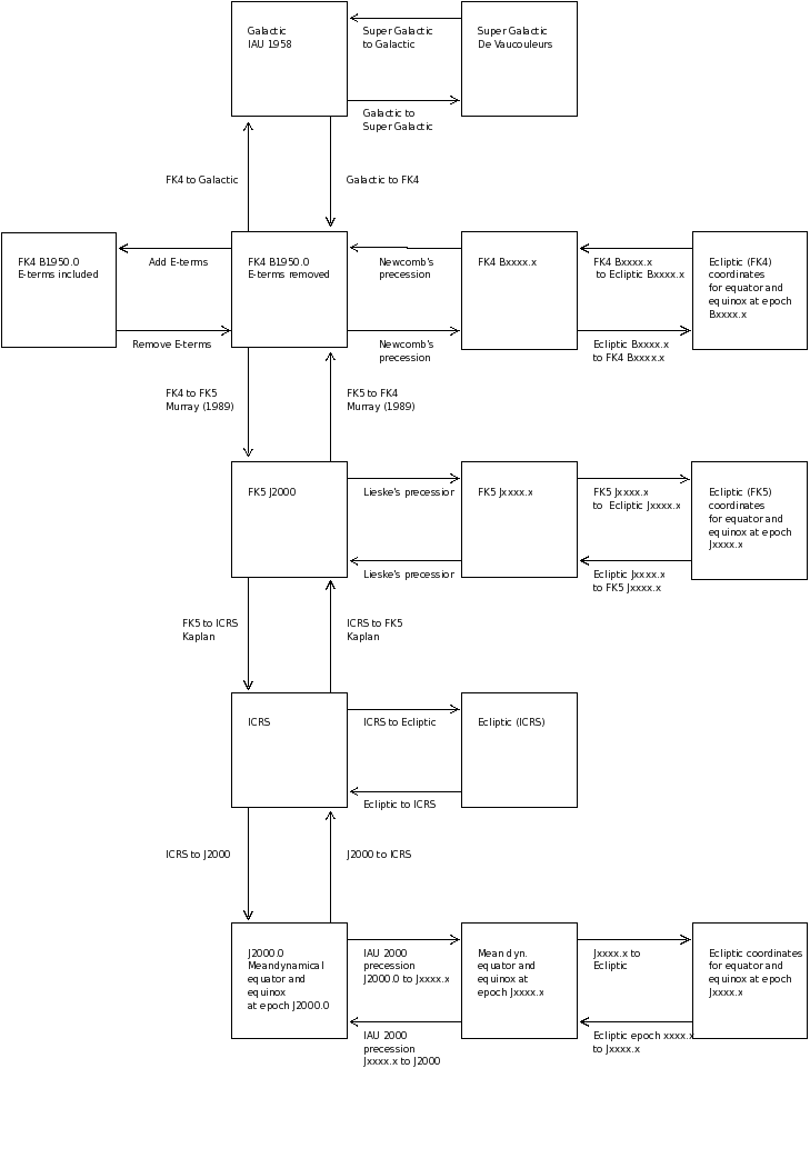
Fig.3 – Schematic overview of all possible transformations in celestial.
Note
The figure illustrates that for each transformation from FK4 and for each transformation to FK4, the E-terms are processed. This has been motivated for transformations between FK4 and FK5. For galactic coordinates we assume that the galactic pole was given in FK4-NO-E. The difference between the position in FK4 and FK4-NO-E is much smaller than the errors in the position of the galactic pole which is the motivation to use FK4-NO-E as the starting point (which means that we use improved mean places anyhow).
Defaults in relation to FITS
In FITS the type of world coordinate system (celestial system) is specified in keyword
CTYPE
For equatorial systems, the reference system in FITS is given with
keyword RADESYS
The epoch of the mean equator and equinox is given with FITS keyword
EPOCH (deprecated) or EQUINOX
For ecliptic and equatorial systems, some rules are set:
- Epoch is sometimes used to refer to the time of observation so if both keywords are given,
EQUINOXtakes preferenceEQUINOXalso applies to ecliptic coordinates- For
RADESYSvalues of FK4 and FK4-NO-E any stated equinox is BesselianRADESYSalso applies to ecliptic coordinates- If for FK4 neither
EQUINOXorEPOCHare given, a default of 1950 will be taken- For
RADESYSvalue of FK5 the stated equinox is Julian- If only
EQUINOXis given and notRADESYSthen the reference system defaults to FK4 ifEQUINOX< 1984 and it defaults to FK5 ifEQUINOX> 1984- If both
RADESYSandEQUINOXare absent thenRADESYSdefaults to ICRS- A date of observation is given in keywords
MJD-OBSorDATE-OBS
Glossary
Most of the definitions are from the reference below or from various web sources.
- Besselian to Julian epoch
- B = 1900.0 + (Julian date - 2415020.31352) / 365.242198781 (according to IAU).
- Epoch
- Instant of time.
- Epoch B1950
- Mean orientation of the earth’s equator and ecliptic at the beginning of the year 1950 (1950,01,01, 12h). It is tied to the sky by star coordinates in the FK4 catalog.
- Epoch J2000
- Mean orientation of the earth’s equator and ecliptic at the beginning of the year 2000 (2000,01,01, 12h). It is tied to the sky by star coordinates in the FK5 catalog.
- Equinox
- An equinox is a moment in time when the center of the Sun can be observed to be directly above the Earth’s equator. At an equinox, the Sun is at one of two opposite points on the celestial sphere where the celestial equator (i.e. declination 0) and the ecliptic intersect (Vernal and autumnal points).
- Equinox of the date
- Means that the equinox is the same as the epoch.
- Ecliptic
- The Ecliptic is the plane of the Earth’s orbit, projected onto the sky. Ecliptic coordinates are a spherical coordinate system referred to the ecliptic and expressed in terms of “Ecliptic latitude” and “Ecliptic longitude”. By implication, Ecliptic coordinates are also referred to a specific “Equinox”
- Equator: true equator of a date
- Is the plane perpendicular to direction of the celestial pole.
- Equator: mean equator of a date
- Is deduced from the true equator of the date by a transformation given by the nutation theory.
- Fiducial point
- A point on a scale used for reference or comparison purposes. If the plane of the ecliptic and the plane of the equator is used as lanes of reference, the equinox is used as fiducial point.
- FK4
- FundamentalKatalog 4. The 4th fundamental catalog. The FK4 is an equatorial coordinate system (coordinate system linked to the Earth) based on its B1950 position. The units used for time specification is the Besselian Year (Fricke & Kopff 1963). See also: Fricke, W., & Kopff, A. 1963, Fourth Fundamental Katalog (FK4), Veroeff. Astron. Rechen-Inst. Heidelb. No. 10. The FK4 system is not inertial. There is a small but significant rotation relative to distant objects. So, besides the equinox, an epoch is required to specify when the mean place was correct.
- FK5
- FundamentalKatalog 5. Based on J2000 positions. The units used for time specification is the Julian year.
- Galactic coordinates
- The galactic coordinate system is a spherical reference system on the sky where the origin is close to the apparent center of the Milky Way, and the “equator” is aligned to the galactic plane.
- ICRS
- Current astrometric observations and measurements should now be made in the International Celestial Reference System (ICRS) The best optical realization of the ICRF currently available is the Hipparcos catalogue. The Hipparcos frame is aligned to the ICRF to within about 0.5 mas For reasons of continuity and convenience, the orientation of the new ICRS frame was set up to have a close match to FK5 J2000. See for example: http://aa.usno.navy.mil/faq/docs/ICRS_doc.php
- mas
- milliarcsecond (\(10^{-3}\) arcsec).
- Obliquity (of the Ecliptic)
- This term refers to the angle the plane of the equator makes with the plane of the Earth’s orbit.
- Precession
- The orientation of the Earth’s axis is slowly but continuously changing, tracing out a conical shape in a cycle of approximately 25,765 years This change is caused by the gravitational forces (mainly Sun and Moon).
- Reference frame
- A reference frame consists of a set of identifiable fiducial points on the sky along with their coordinates, which serves as the practical realization of a reference system.
- Reference system
- A reference system is the complete specification of how a celestial coordinate system is to be formed. It defines the origin and fundamental planes (or axes) of the coordinate system. It also specifies all of the constants, models, and algorithms used to transform between observable quantities and reference data that conform to the system.
References
| [Aoki1] | Aoki, S., Soma, M., Kinoshita, H., Inoue, K., 1983. Conversion matrix of epoch B 1950.0 FK4-based positions of stars to epoch J 2000.0 positions in accordance with the new IAU resolutions, Astron. Astrophys. 128, p.263-267, 1983, ADS Abstract Service 1983 |
| [Aoki2] | Aoki, S. et al, 1986. The Conversion from the B1950 FK4 Based Position to the J2000 Position of Celestial Objects, Astrometric Techniques: IAU SYmp:109 Florida p.123, 1986, ADS Abstract Service 1986 |
| [Blaauw] | Blaauw, A.; Gum, C. S.; Pawsey, J. L.; Westerhout, G., 1959, Note: Definition of the New I.A.U. System of Galactic Co-Ordinates Astrophysical Journal, vol. 130, p.702, ADS Abstract Service 1959 |
| [Brouw] | Brouw, W.N., 1974. Synthesis Radio Telescope Project; The SRT Reduction Program, Internal Technical Report ITR 78 about the Standard Reduction Program for the Westerbork Synthesis Radio Telescope, Astr. Observatory, Leiden, Netherlands |
| [Calabr] | Calabretta, M.R., Greisen, E.W., 2002 Representations of celestial coordinates in FITS Astronomy and Astrophysics, v.395, p.1077-1122 (2002). PDF version at http://www.atnf.csiro.au/people/mcalabre/WCS/ |
| [Corwin] | Corwin, H. G.; de Vaucouleurs, A.; de Vaucouleurs, G., 1994. Southern Galaxy Catalogue (SGC), VizieR On-line Data Catalog: VII/116. Originally published in: 1985MAUTx...4....1C, RC3 - Third Reference Catalog of Bright Galaxies |
| [Cotton] | Cotton, W. D.; Condon, J. J.; Arbizzani, E. , 1999. Arcsecond Positions of UGC Galaxies, The Astrophysical Journal Supplement Series, Volume 125, Issue 2, p.409-412 ADS Abstract Service 1999 |
| [Diebel] | Diebel, J, 2006.
Representing Attitude: Euler Angles, Quaternions, and Rotation Vectors
(local copy) |
| [Hering] | Hering, R.; Walter, H. G., 1998. Updating of B1950 radio star positions by means of J2000 calibrators. International Spring Meeting of the Astronomische Gesellschaft: The message of the angles - astrometry from 1798 to 1998, p.198 - 200, http://www.astro.uni-bonn.de/~pbrosche/aa/acta/vol03/acta03_198.html |
| [Hilton] | Hilton, J.L.; Hohenkerk, C. Y., 2004. Rotation matrix from the mean dynamical equator and equinox at J2000.0 to the ICRS Astronomy and Astrophysics, v.413, p.765-770 (2004). ADS Abstract Service 2004 |
| [Kaplan] | Kaplan, G.H., 2005. The IAU Resolutions on Astronomical Reference systems, Time scales, and Earth Rotation Models, US Naval Observatory, Circular No. 179, http://aa.usno.navy.mil/publications/docs/Circular_179.pdf |
| [Lieske1] | Lieske, J. H.; Lederle, T.; Fricke, W.; Morando, B., 1977. Expressions for the precession quantities based upon the IAU /1976/ system of astronomical constants, Astronomy and Astrophysics, vol. 58, no. 1-2, June 1977, p. 1-16 ADS Abstract Service 1977 |
| [Lieske2] | Lieske, J.H., 1979. Precession matrix based on IAU 1976 system of astronomical constants Astronomy and Astrophysics, vol. 73, no. 3, Mar. 1979, p.282-284, ADS Abstract Service 1979 |
| [Murray] | (1, 2, 3) Murray, C.A., 1989. The transformation of coordinates between systems of B1950.0 and J2000.0 and the principal galactic axes referred to J2000.0, Astron. Astrophys, 218, p.325-329, ADS Abstract Service 1989 |
| [Poppe] | Poppe P.C.R., Martin, V.A.F., 2005. Sobre as Bases de Referencia Celeste (On the celestial reference frames), Sitientibus Serie Ciencias Fisicas 01: 30-38 (2005), http://www2.uefs.br/depfis/sitientibus/vol1/Vera_Main-SPSS.pdf |
| [Scott] | Scott F.P., Hughes J.A. , Computation of Apparent Places for the Southern Reference Star Program, The Astronomical Journal, Vol 69, Number 5, 1964, p.368-371, ADS Abstract Service 1964 |
| [Seidel] | Seidelmann, P.K., 1992. Explanatory Supplement to the Astronomical Almanac, University Science Books |
| [Smart] | Smart, W.M., 1931, Sixth ed. 1977, reprint 1990. Textbook on Spherical Astronomy, Sixth Edition, Revised by R.M. Green, Cambridge University Press |
| [Smith] | Smith, C. A.; Kaplan, G. H.; Hughes, J. A.; Seidelmann, P. K.; Yallop, B. D.; Hohenkerk, C. Y., 1989. Mean and apparent place computations in the new IAU system. I - The transformation of astrometric catalog systems to the equinox J2000.0. II - Transformation of mean star places from FK4 B1950.0 to FK5 J2000.0 using matrices in 6-space, ADS Abstract Service 1989II |
| [Soma] | Soma, M., Aoki, S. 1990. Transformation of the Mean Place from FK4 to FK5, Inertial Coordinate System Of/ Sky: IAU SYMP.141 p.131, 1989, ADS Abstract Service 1990 |
| [Wallace1] | Wallace, P. T., 1994. The SLALIB Library , Astronomical Data Analysis Software and Systems III, A.S.P. Conference Series, Vol. 61, 1994, Dennis R. Crabtree, R.J. Hanisch, and Jeannette Barnes, eds., p.481. |
| [Wallace2] | Wallace, P. (chair), IAU SOFA, IAU, 2007, SOFA Tools for Earth Attitude sofa_pn.pdf and also: ADS Abstract Service 1994 |
| [Wallace3] | Wallace, P. T., 2005. SLALIB – Positional Astronomy Library 2.5-3 Programmer’s Manual, Manual |
| [Yallop] | Yallop, B. D.; Hohenkerk, C. Y.; Smith, C. A.; Kaplan, G. H.; Hughes, J. A.; Seidelmann, P. K., 1989. Mean and apparent place computations in the new IAU system II. Transformation of mean star places from FK4 B1950.0 to FK5 J2000.0 using matrices in 6-space, Astron. Journal, 97, Number 1, January 1989, ADS Abstract Service 1989 III |